The Amarantos Ritual - 07 - Vortex VFX Tutorial

Intro

Creating Polar Coordinates / Circular Distortion in UE5.

In this tutorial we cover how to make an Unreal 5 material shader VFX. There are two other parts in this tutorial series. In “Part One” we created the base static geometry needed for the VFX. Then in “Part Two” we created some textured noises in Substance Designer.

In this third part, we will use the textures created inside an Unreal 5 Material Graph. First we will created the “parent” material, then we will copy an instance of it and tweak the values of the different scalars and parameters and get the visual that we see below.

Software that we will be using:

Unreal Engine 5
Blender
Substance Designer

Tip:

In this third part, I will be created the parent material in Unreal Engine 5. If your project is in Unreal Engine 4, you can still follow. The tutorial does not use any material graph nodes or features that are locked to UE5. Everything is available in UE4 as well.

If you are curious for the exact version of my engine, I will be using UE5.3. You can use any previous ones though, as already mentioned above.

As usual, before we go into UE5 and start working, lets see a reminder of what the end result will be:

Videos Preview

(Youtube embedded video above, showcasing the final vortex VFX we will be creating.)

The previous two parts of the tutorial we made the geometry and the textures, now we will create the main part - the shader.

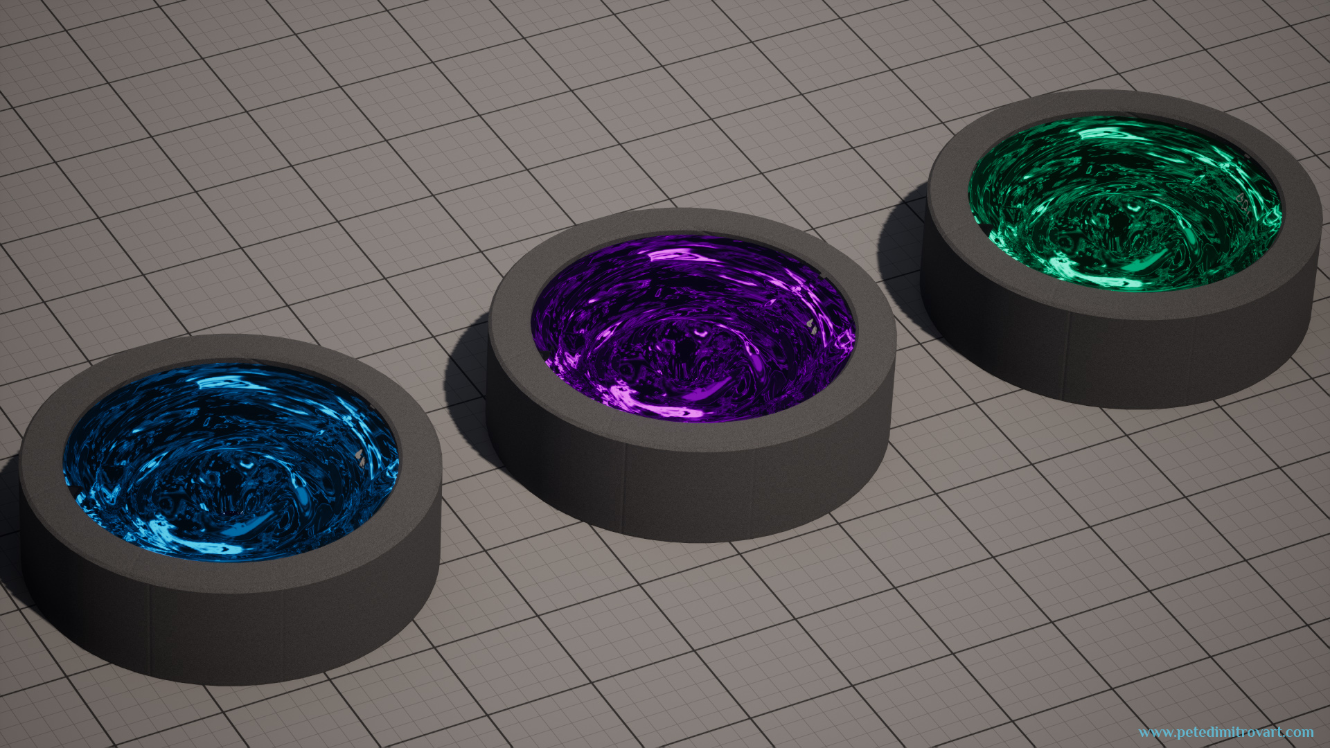
(Youtube embedded video above. Shows the VFX basin duplicated three times. One is blue, the other is purple, the last one is green.)

Screenshots Preview

As seen before, here are screenshot previews:

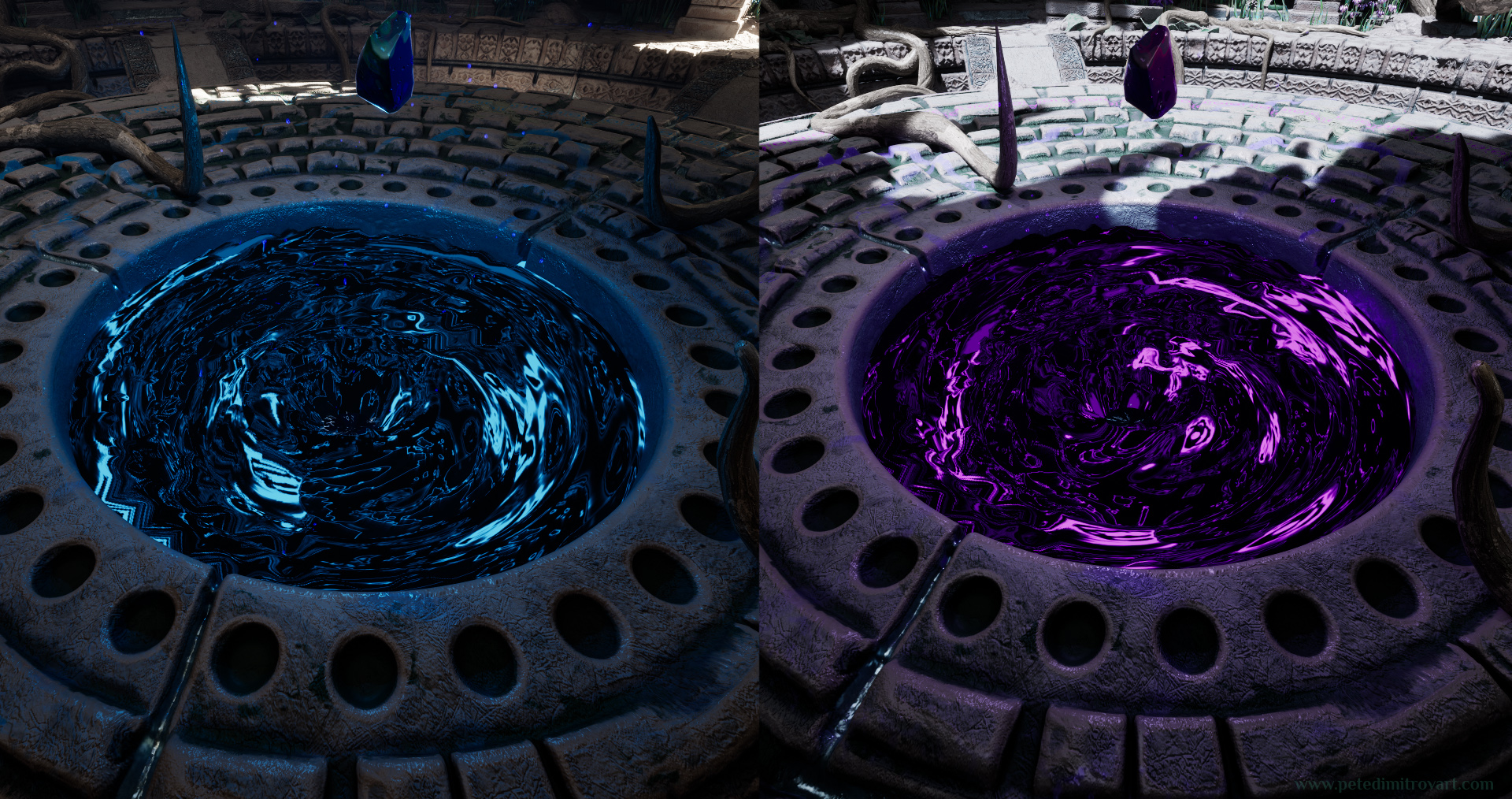
$Two vortex VFXs next to one another. One is tinted in black and blue. The other is tinted in purple and blue. Their surface has long stripes of emissive color but also a lot of distortion as if its seen through refraction. Unreal 5 screenshots.$

As said in the previous entries, we are making only the VFX, not the rest of the room or art, but you can read about the creation process of those over here.

Another angle showcasing the vortex basin VFX. This time its 3 of them. A blue, purple and then a green one. They are seen in a placeholder scene with grid materials. The camera is from very, very far away and unrealistically small Field of View (or otherwise large Focal Length), reducing the perspective and showcasing the props as if from an orthographic view.

Polar Coordinates

Before we get into creating our UE5 material graph, I want to take a moment and talk about the shader itself. The technique we are after is UV distortion and tiling that with a panner makes a movement towards a central point. Like a vortex. This effect is accomplished through “polar coordinates”. It is all UV coordinates distortion. We feed in an ordinary tiling texture and we manipulate its UVs to get a circular, inwards motion (or outwards, we can change direction just through one parameter).

A very simple, short explanation of what exactly we are doing is the following. We take linear direction coordinates: on the U and V axis and we use maths to distort them into circular coordinates.

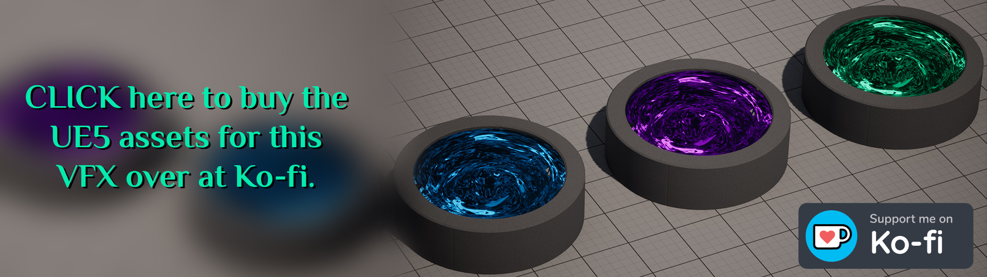
The material shader, seen in an orthographic camera screenshot from Unreal 5. There are three shapes. One is flat plane, second is a vortex basin, third one is the same. First two have black and white, liquid-like texturing. Third one is tinted in green.

If you would like to buy the work files behind this tutorial series, follow the link by clicking the image below.

In Other Games

The above explained technique is incredibly powerful. It’s not hard to create and its not very demanding resources wise (it scales on the GPU, which is always a good thing for performance in games). As such its very commonly seen in games. That is both in old and new titles. Both in AAA and indie games.

As such I wanted to show you a few examples that I came across randomly, without searching, while I was playing some games recently. That will help you see the elegance of the technique we are about to use.

Diablo IV

In Diablo 4 that I’ve been playing quite a bit at the time of writing this, there are a few world bosses. The map gets a pin with a timer that gives you 30 minutes to get to a special zone where the boss entity will spawn. Lots of players gather there and if you are early you get to see a few different animations and effects that show the “preparation” of the spawning of the giant enemy you are about to face.

When Ashava the Pestilent is about to spawn, their presence in Saraan Caldera is announced by this large, toothed mesh:

Video embedded above. Shows a clip from Diablo 4 that shows a flesh, bones and tooths-like giant 3D mesh. In the middle there is a flat plane with a vortex VFX motion that moves outwards, as if some miasma, tar and poison moves.

If you look past the mesh and its movement, and focus on the middle, you will see a flat plane with a VFX material applied to it. That material is absolutely identical to the one we are making. Its a vortex like motion, panned outwards. The artist at Blizzard have made and applied normal and albedo textures to give it a dark, tar-like appearance. Looks amazing!

Baldur’s Gate 3

Another title I’ve been obsessed with (many of you most likely are as well) is Baldur’s Gate 3.

Another video embed above. Shows four adventurers inside the dark interiors of Moonrise Towers zone. Under their feet is an animated aura VFX. It looks like a bright, chroma and rainbow vortex.

If you look under the feet of my Tiefling Sorcerer in the video above, on the dark floor tiles of Moonrise Towers you will see a bright, white vortex with outwards movement. From time to time it gets a chromatic tint that gives it a subtle rainbow look.

This again is exactly the polar coordinates UV distortion we are making. The difference between this one and ours (and the one in Diablo 4) is that here, the devs at Larian Studios have also put a low opacity mask. That gives the effect a more transparent look.

Material Graph Preview

Lets first see the entire material graph:

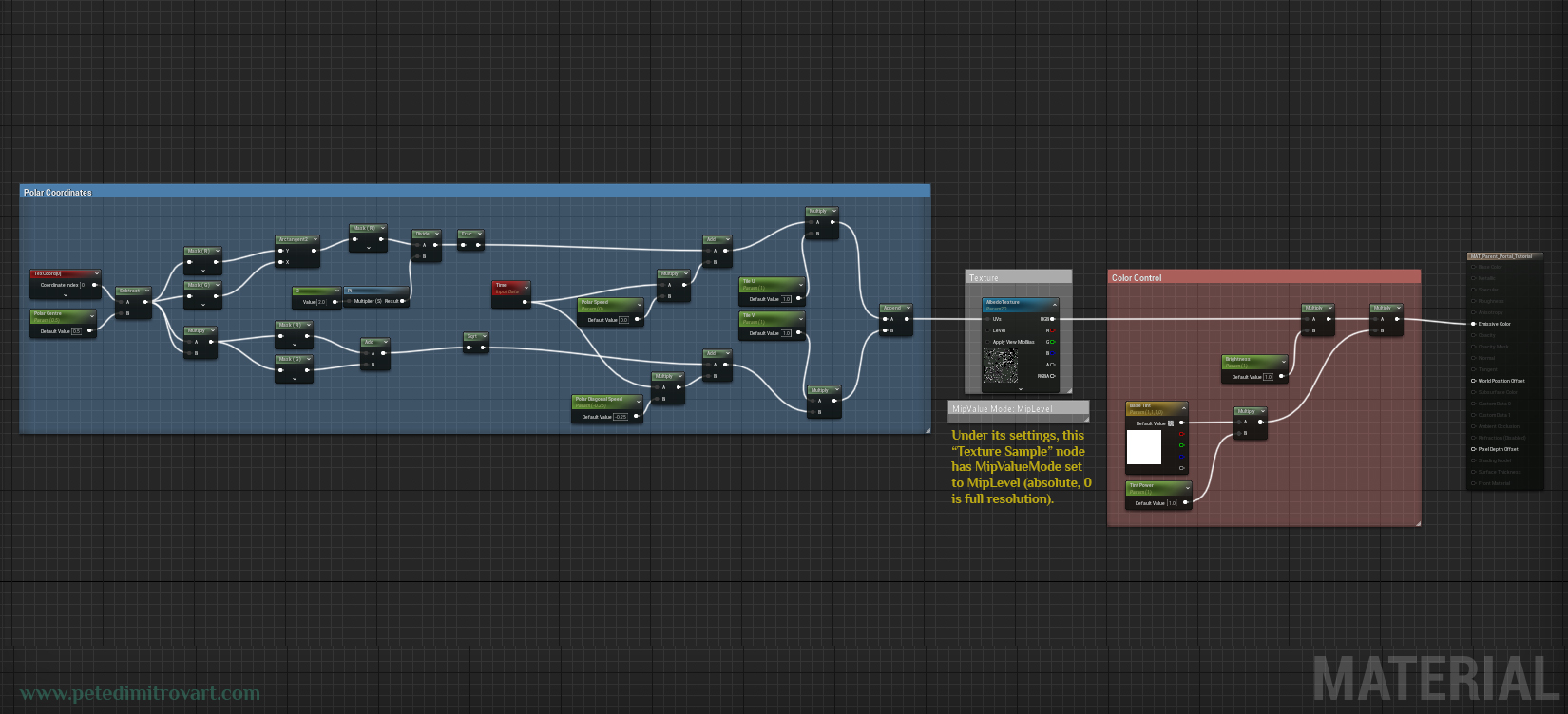
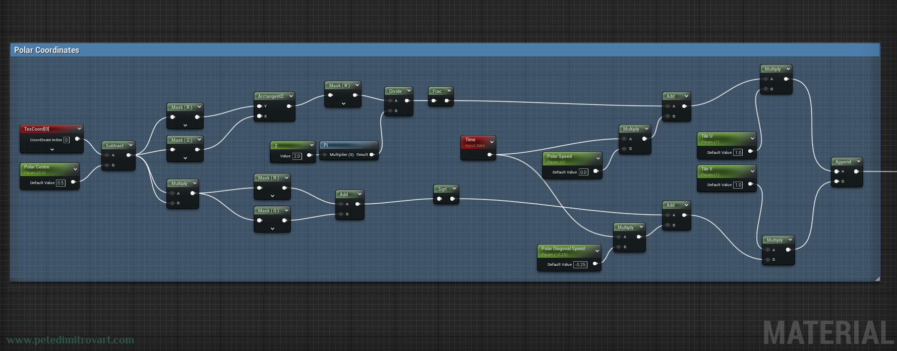
UE5 screenshot of a material graph. Lots of nodes are bundle together and framed into 3 color categories: blue for “Polar Coordinates”, white for “Texture Sample” node and final red group for “Color Control”. The final pin gets connected to the output seen in the right side.

Then lets zoom in for better readability:

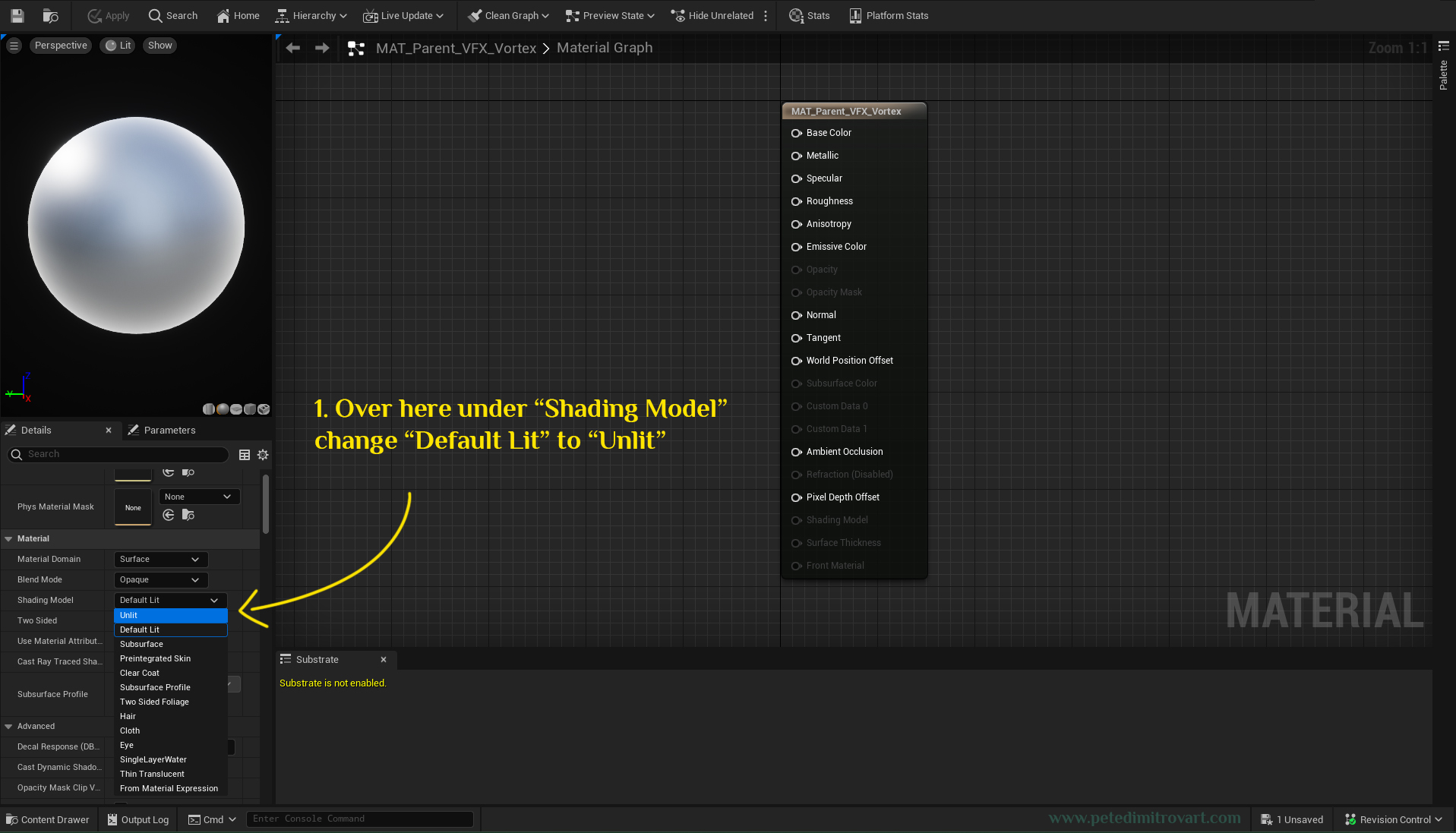
The blue framed group from the previous picture, but now zoomed in.

The gray, white group and the red group, framed and zoomed in. They are seen connected into the final output.

With the output (final node) selected, here are its material settings to the left side of the screenshot:

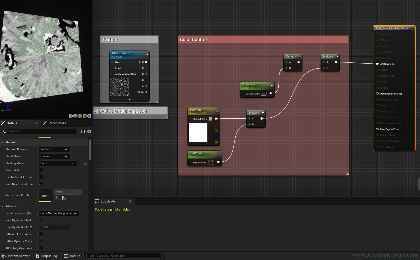
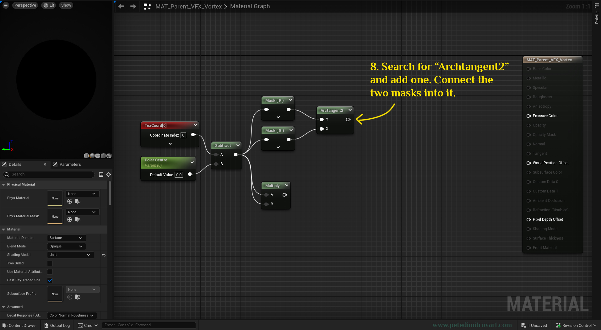
In this UE5 screenshot the material final output is selected. That enables seeing the material settings to the very left. The important ones are transcribed below.

For “Material Domain” we use “Surface. In the “Blend Mode” we go “Opaque”. For “Shading Model” we use “Unlit”. Two Sided is ticked off, Use Material Attributes is off as well. “Cast Ray Traced Shadows” is on and for Subsurface Profile there is nothing. The Advanced settings are left to their default states.

If you only want to get the visual result and are not interested in any technical, mathematical or further detailed explanation behind some of the steps and nodes, you can replicate what you see from the zoomed up pictures above and skip most of the tutorial below.

Lets start from the beginning though:

Creating the Polar Coordinates

Create a “Materials” folder in your project directory. Inside create a “Parents” folder. In there we will create our parent materials from which we will create our instanced materials later on.

Right click in there and make a new material. Name it “MAT_Parent_VFX_Vortex”. Open it. Click the output node and lets tweak the settings, putting them to what we mentioned tiny bit ago:

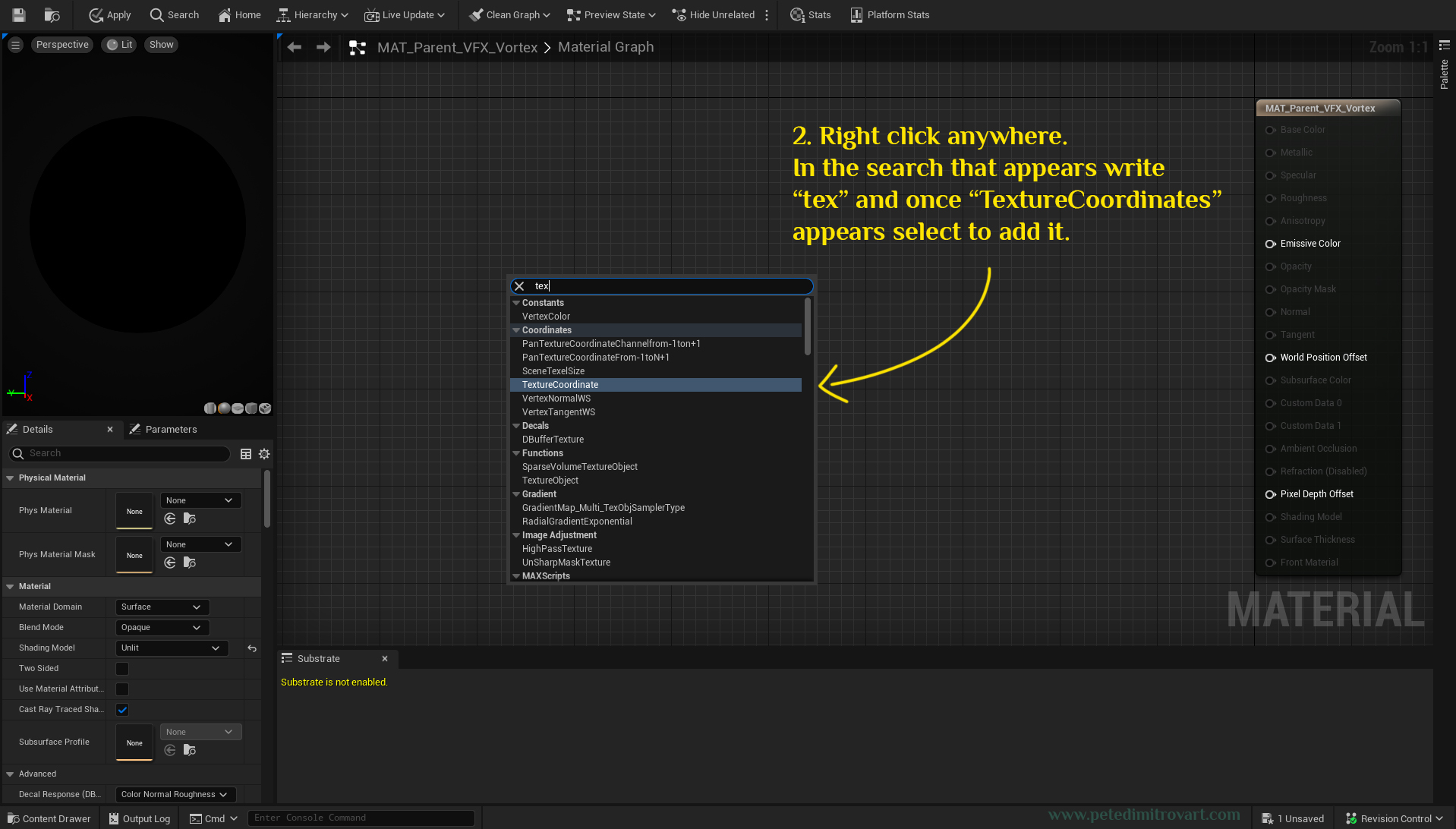
Unreal 5 material graph screenshot. Shows the material settings, to the left, being changed from Shading Model “Default Lit” to “Unlit”.

Right click anywhere. In the search box that appears write “tex” and once “TextureCoordinates” appears, click on it to add it.

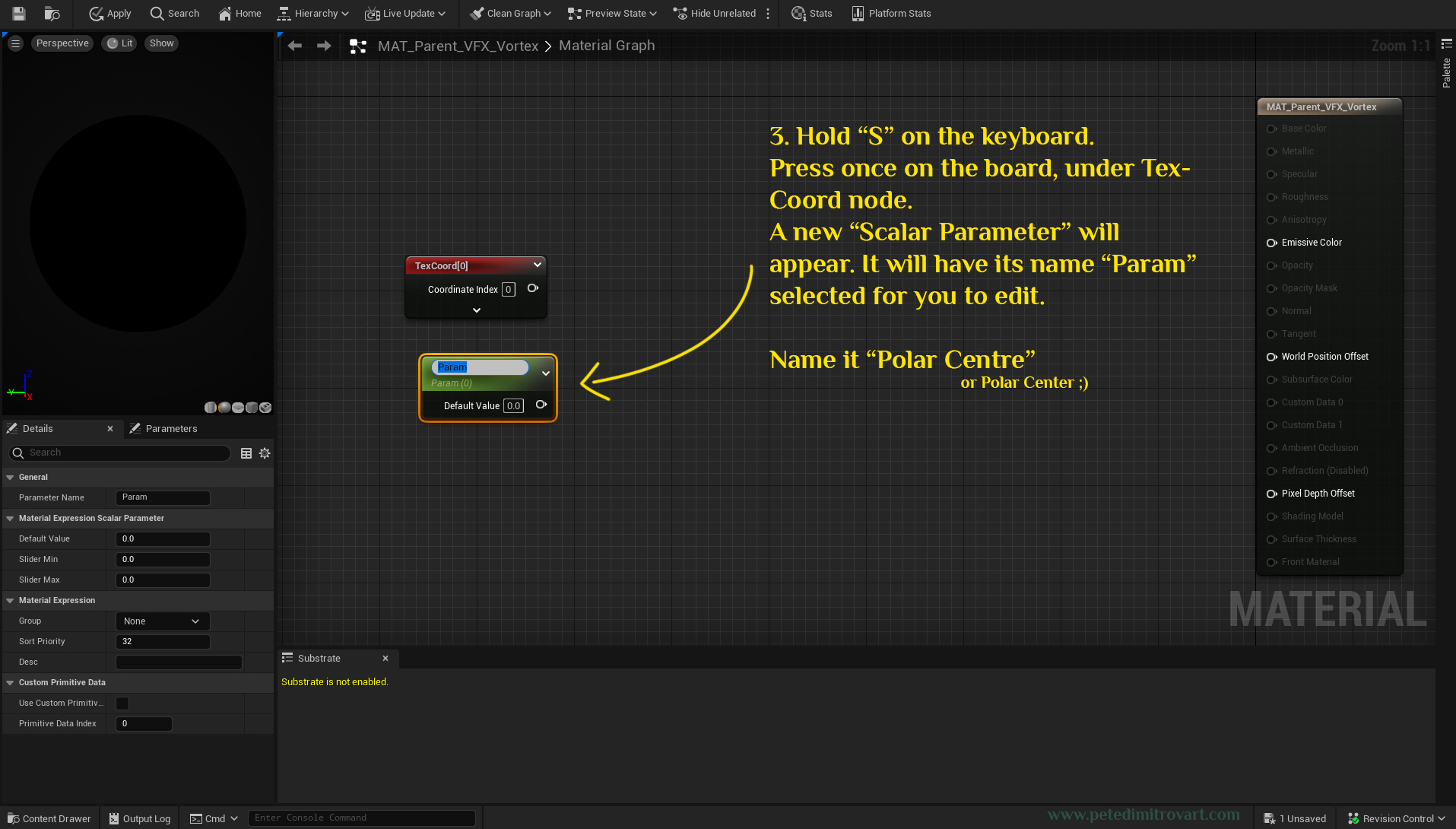
UE5 screenshot showing an open search context menu with “Texture Coordinates” selected.

Hold “S” on the keyboard. Press once on the board, under the newly added TexCoord node. A new “Scalar Parameter” will appear. It will have its name set as “Param”. Edit it and name it “Polar Centre”.

Screenshot like before but now there is a red node added - thats the TexCoord. Under it is added a new scalar parameter (green node).

Component Mask

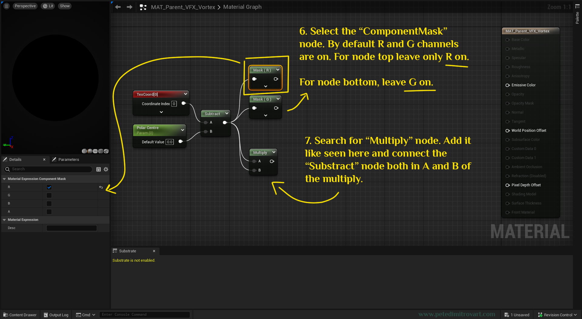
Using the search we explained, find and add “Subtract” node. Connect it like what is seen below. Then search “ComponentMask” and add two of them. We will order and tweak them in the next step.

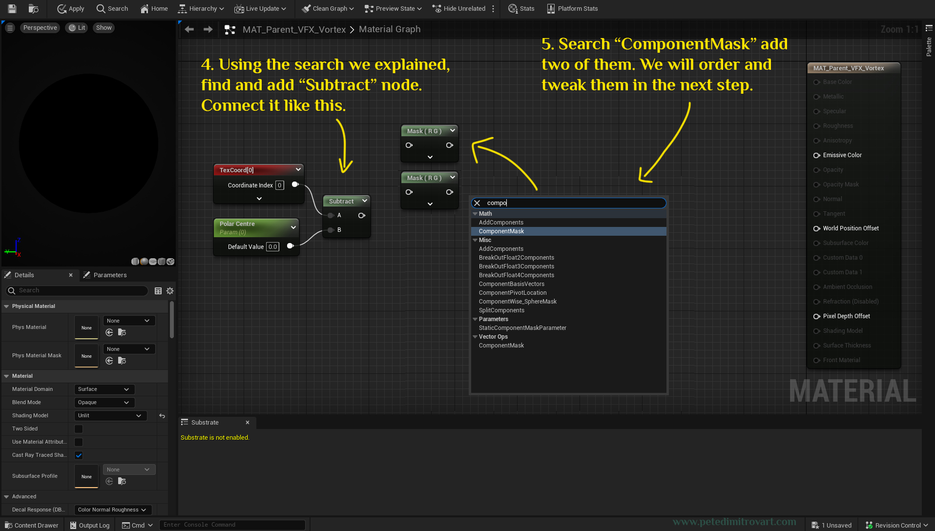
Another shot showing the red and green pines (TexCoord and Polar Centre) being connected to the A and B of a Subtract node. To the right of them are added two Mask ( R G ) nodes.

Select the “ComponentMask” node. By default “R” and “G” channels are on. For node that is on the top row, leave only “R” on. For the node that is at the bottom, leave “G” on. Then search for a “Multiply” node. Add it like seen below (which is both A and B connected to the Subtract).

Image showing one of the Component Mask nodes being selected. From its settings to the left, only R from RGBA is selected. On the Mask node below it, only G is left on. Then under them is added a Multiply node connected both in A and B into Subtract.

Arctangent2

Search for “Arctangent2” and add one. Connect the two masks into it.

Screenshot showing an Arctangent2 node added right after Mask R and Mask G. R is connected into the Y and G into the X of the Arctangent2.

Tip:

Arc tangent is an inverse tangent function. We do an inverse tangent function because we are switching from Cartesian coordinates and moving into Polar coordinates. We are doing Arctangent2 instead of Arctangent because we are dealing with a coordinates system split into four quadrants. Arctangent would limit us only into quadrant number one and four. By the end of this tutorial I've linked further reading on the topic.

(If you would like a bit more optimized result, you can replace your Arctangent2 for Arctangent2Fast. It is a node a bit less accurate, but still accurate enough for our visuals to remain the same.)

Pi

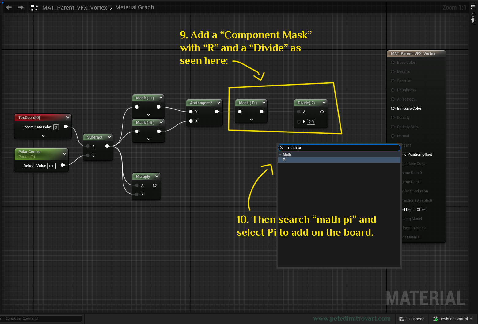
Add a “Component Mask” again, this time change its settings so only “R” channel is on. After it add a “Divide” node and connect the Mask into A. Then search for “math pi” and select Pi to add on the board.

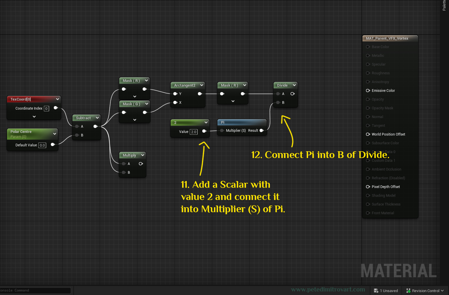
Another shot that shows adding a new component mask, right after Arctangent2. Then its followed by adding Divide right after Mask “R”. The image then shows searching for “math pi” and adding a “Pi” node (seen in next image).

Add a Scalar Parameter with a value of 2 and connect it into Multiplier (S) input of the Pi node. Connect the Pi output into the B input of Divide node.

Image showing a scalar parameter with value of 2 being connected into Pi and then Pi (blue node) is connected into the B input of a Divide node. Yellow text is transcribed above.

Tip:

Let's say you are recreating this in Unity in Shader Graph or in Amplify Shader Editor. Because you totally could, all nodes and functions exist over there, no matter it is another engine. If for some reason Pi is not defined in whatever package you have, you could just add a new scalar parameter and give it a value of == 6.2831 which would be correct enough approximation of 2 x Pi for the shader to work well.

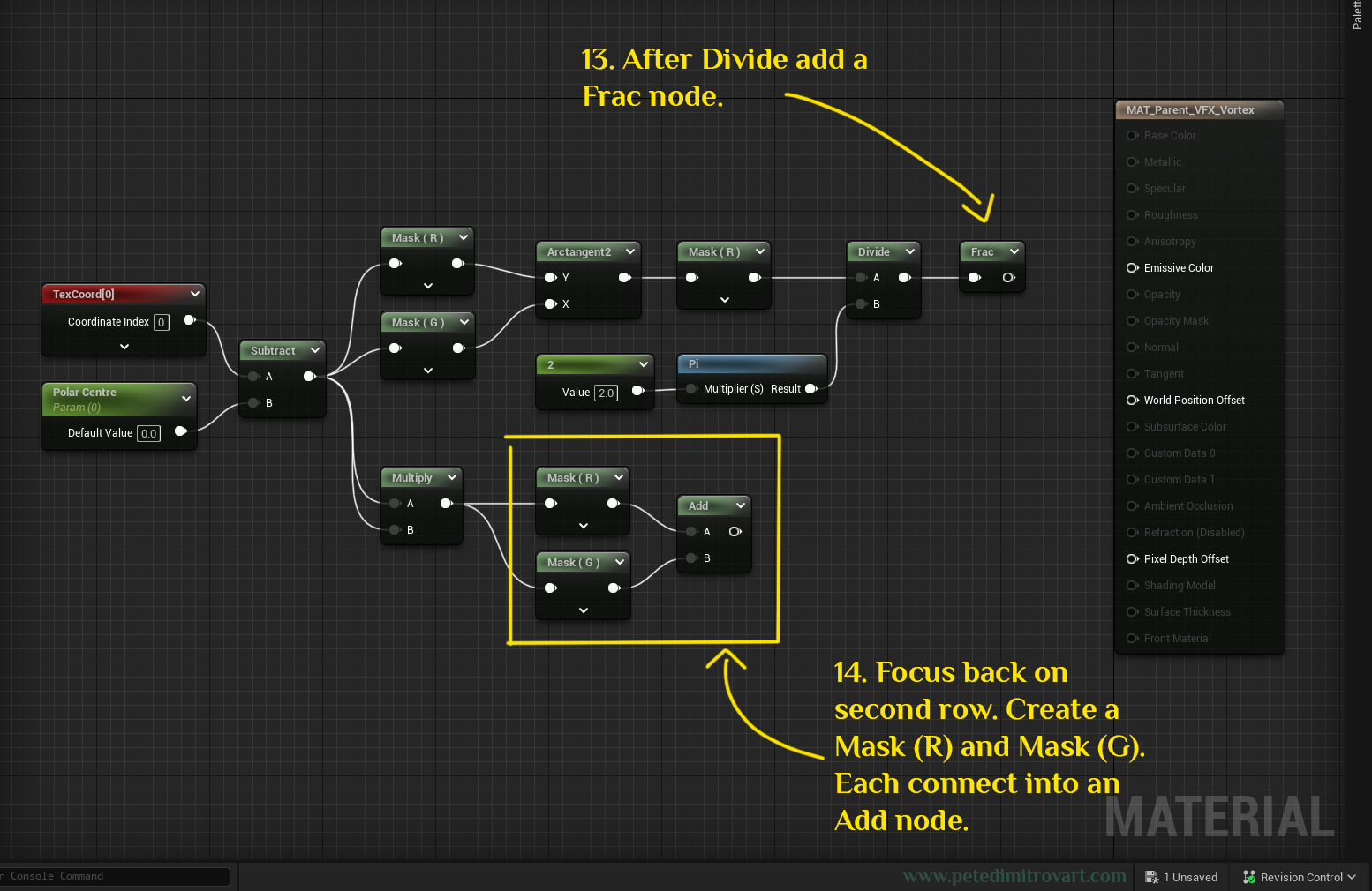
Frac

After the “Divide” node, add a “Frac” node. Now take a look at the lower row, right after the “Multiply” node. Create a Mask (R) and Mask (G) nodes. Connect both of them into an “Add” node.

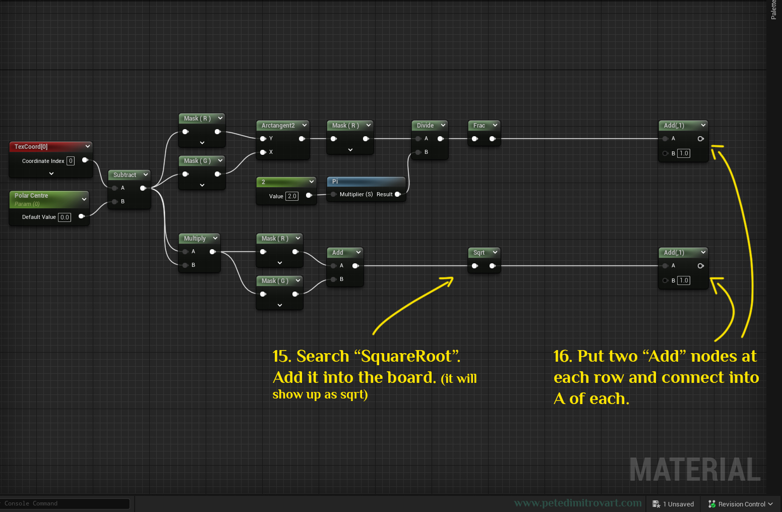
Screenshot showing the nodes board with a “Frac” node added on top row and two Mask and an Add node added to the second row. Text is transcribed above.

Search for “SquareRoot”. Add it into the board (it will show up as “Sqrt”). Now put two “Add” nodes at each row and connect into “A” of each.

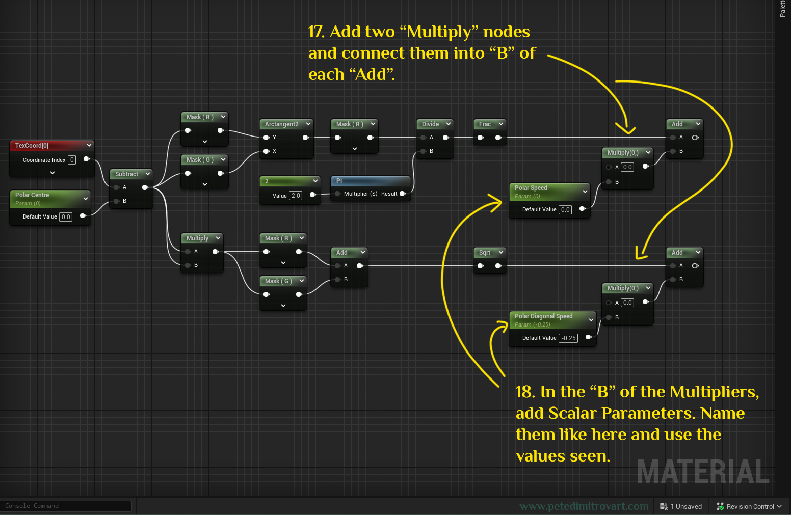
Image showing the addition of a Sqrt node at the bottom. Then both on top and bottom we include new “Add” nodes and connect into the A input of each.

Add two “Multiply” nodes and connect them into “B” of each “Add”. In the “B” of the multipliers, add new Scalar Parameters. Name them “Polar Speed” for top row and “Polar Diagonal Speed” for bottom row.

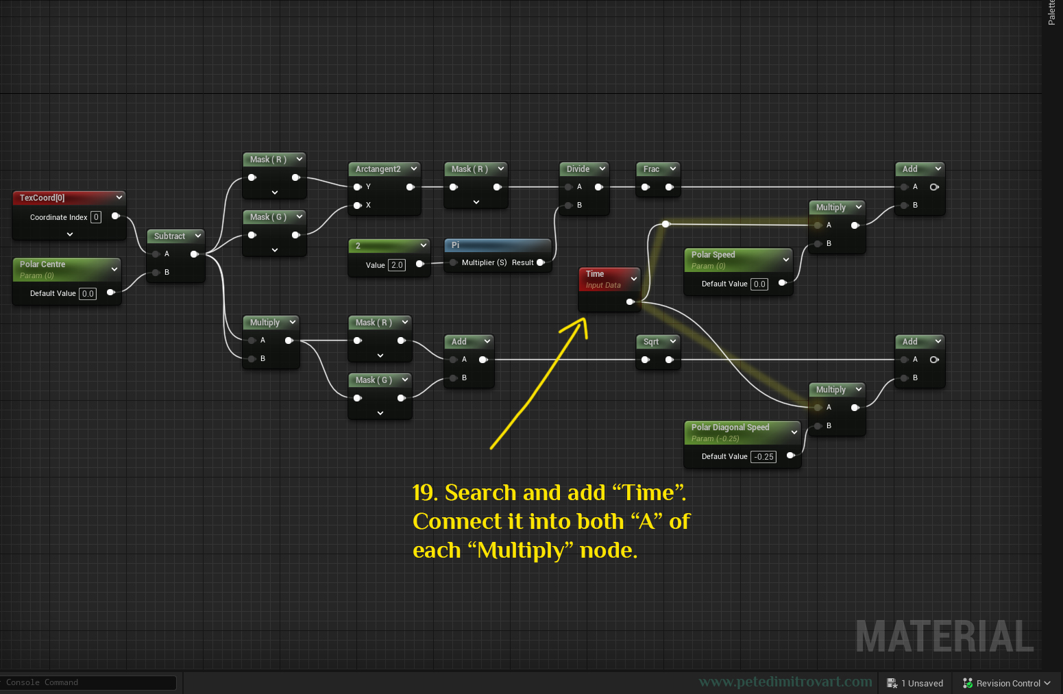
Material graph screenshot showcasing adding two Multiply nodes. Then in the B of each we add new scalar parameters (seen as green color nodes).

Time

Search for “Time” node and add it. Connect it into both “A"s of each “Multiply” node (as seen in picture below).

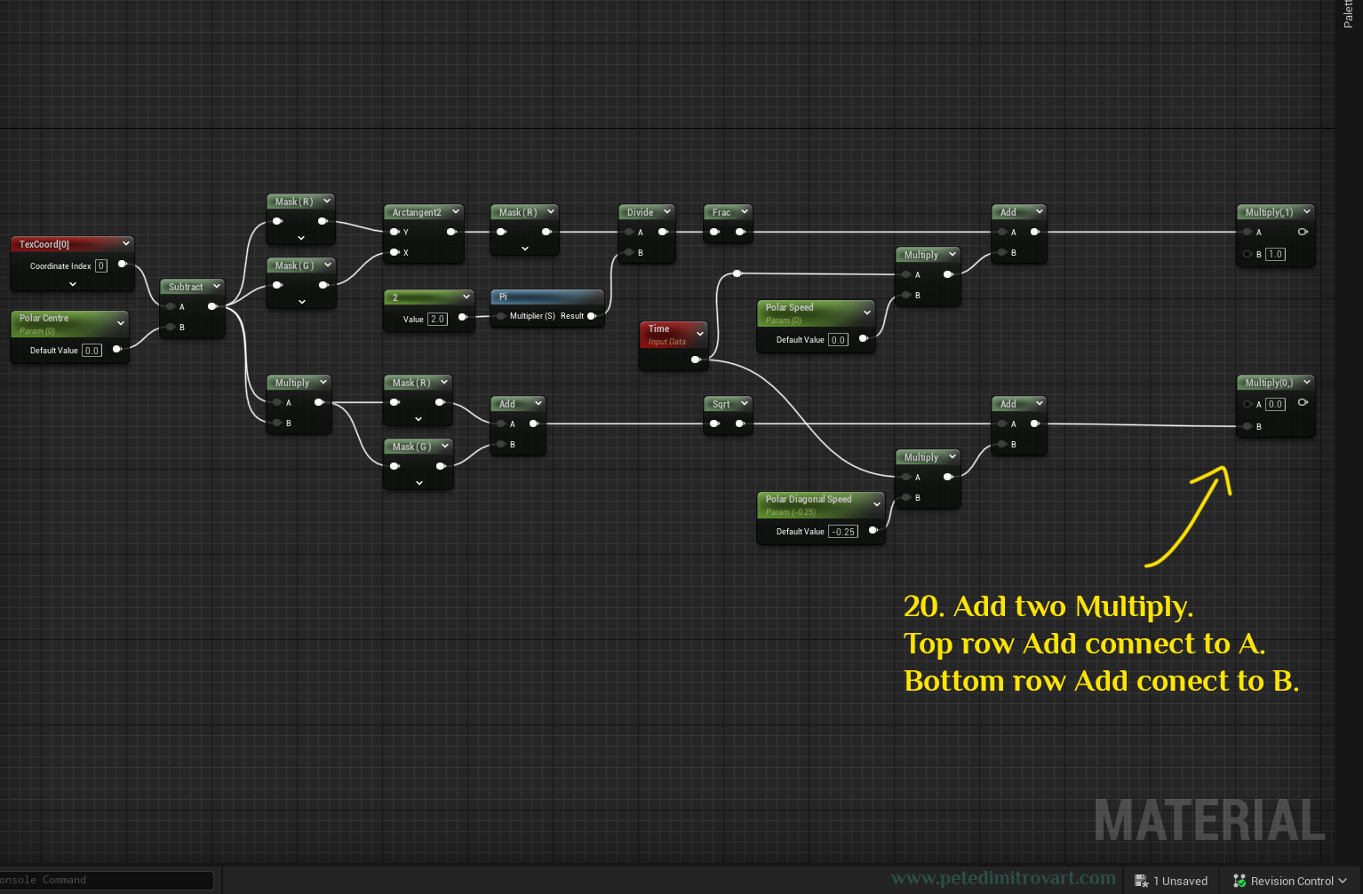
Screenshot showing a new “Time” node, as seen in red color, added and connected to both Multiplies.

Add two “Multiply” nodes. The previous “Add” node seen on top row, connect into A of Multiply top. The bottom “Add” node, connect to “B” of the new, secondary “Multiply” on that row.

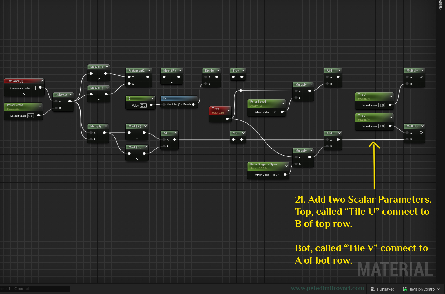
Shot showcasing adding two new multiply nodes at the end of each row. Then the previous Add nodes connect into the A and B of top and bottom multiply.

Add two new Scalar Parameters. Top one call “Tile U” and connect to “B” of top row Multiply. Bottom one call “Tile V” and connect to the “A” of bottom row Multiply.

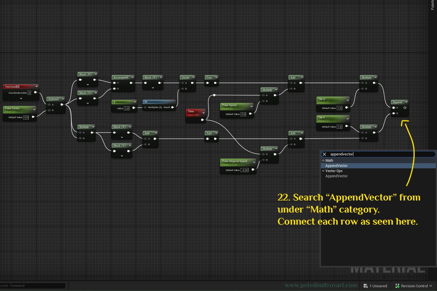
Image shows adding two new scalar parameters, seen in green color, named Tile U and Tile V. Each connects into the B and A of top and bottom Multiply nodes.

Search for “AppendVector” from under “Math” category. Add it to the board. Connect each row as seen here.

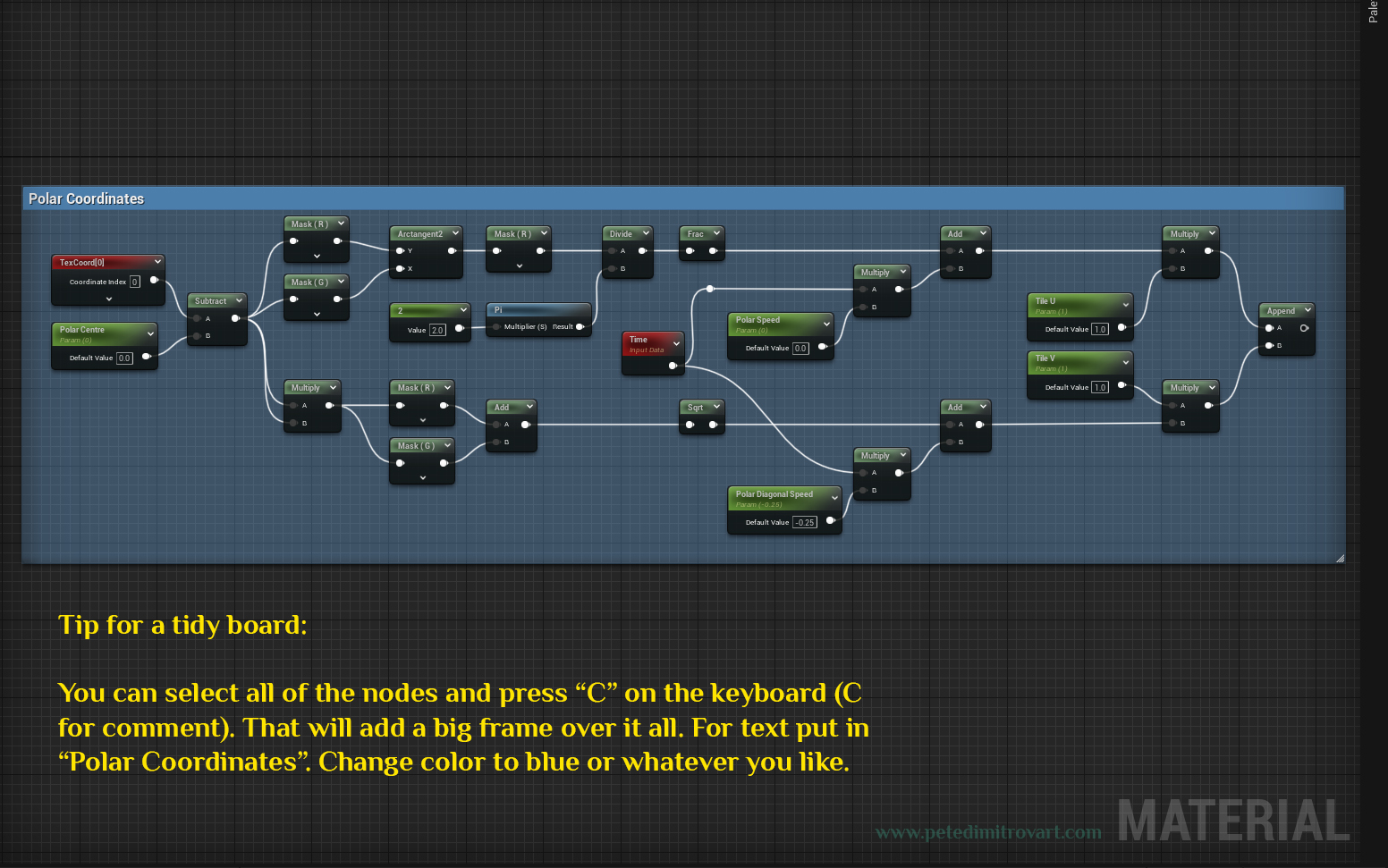
Screenshot where we search “AppendVector” and see it highlighted and show up in search under “Math”. We then add that node right after the previous two Multiply nodes from each row and add each into A and B of “Append”.

Tip for a tidy board:

You can select all of the nodes and press “C” on the keyboard (C stands for Comment in this case). That will add a big frame over it all. For text put in “Polar Coordinates”. Change the color to blue or whatever you like.

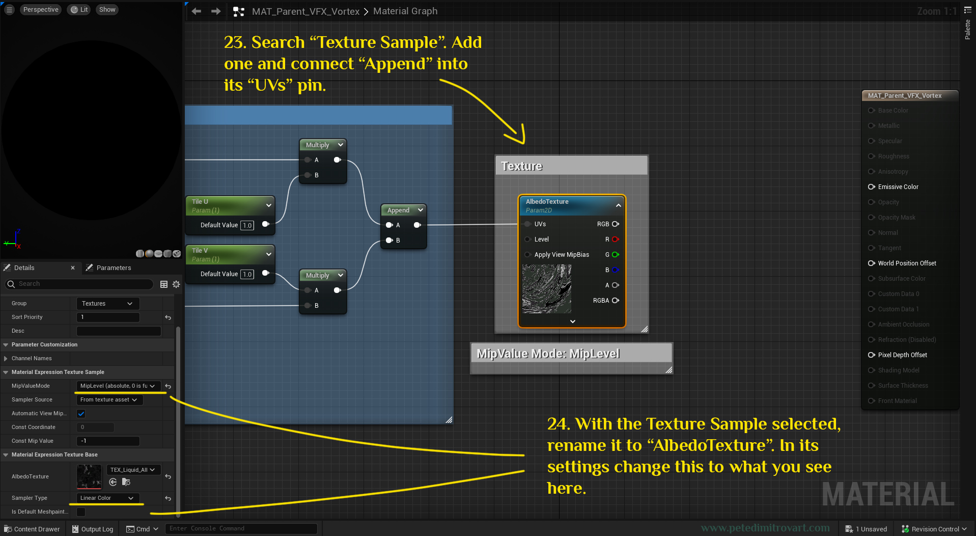
Zoomed out picture of the graph board. It shows all of the nodes we placed and created in all of the previous steps. Its all framed in a blue comment.

Focus on the right side of the previous work, right after the “Append”.

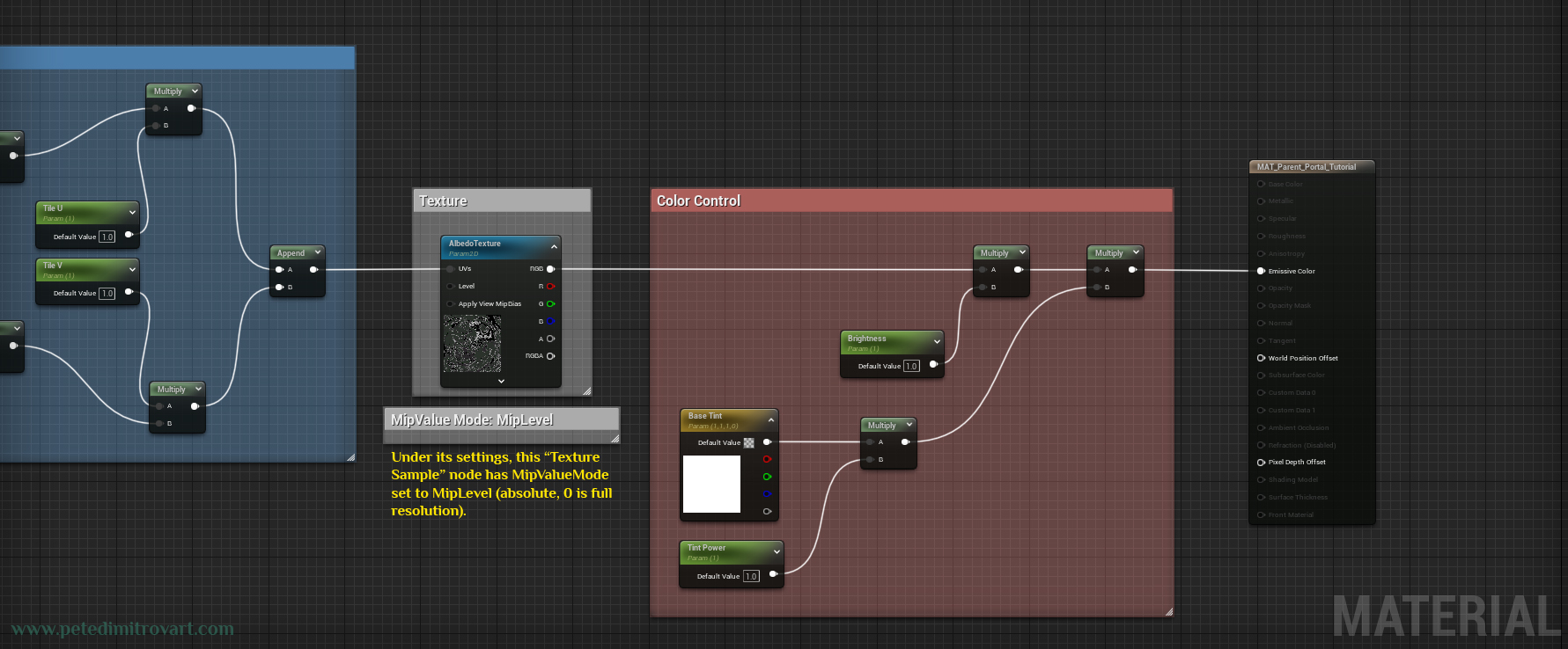
Search “Texture Sample”. Add one and connect “Append” into its “UVs” pin. With the “Texture Sample” selected, rename it to “AlbedoTexture”. In its settings change the following: MipValueMode: MipLevel (absolute, 0 is full resolution). Sampler Type: Linear Color. (these are pointed in the image below).

Image showing the adding of a new Texture Sample node. It’s renamed to AlbedoTexture and the previous append node connects to its UVs. Then two settings for the texture sample node are pointed out and changed as described in the paragraph above.

Color Control

Lets create the final part of the shader. It will be a bunch of new nodes that we will then frame into a red comment box, as seen below.

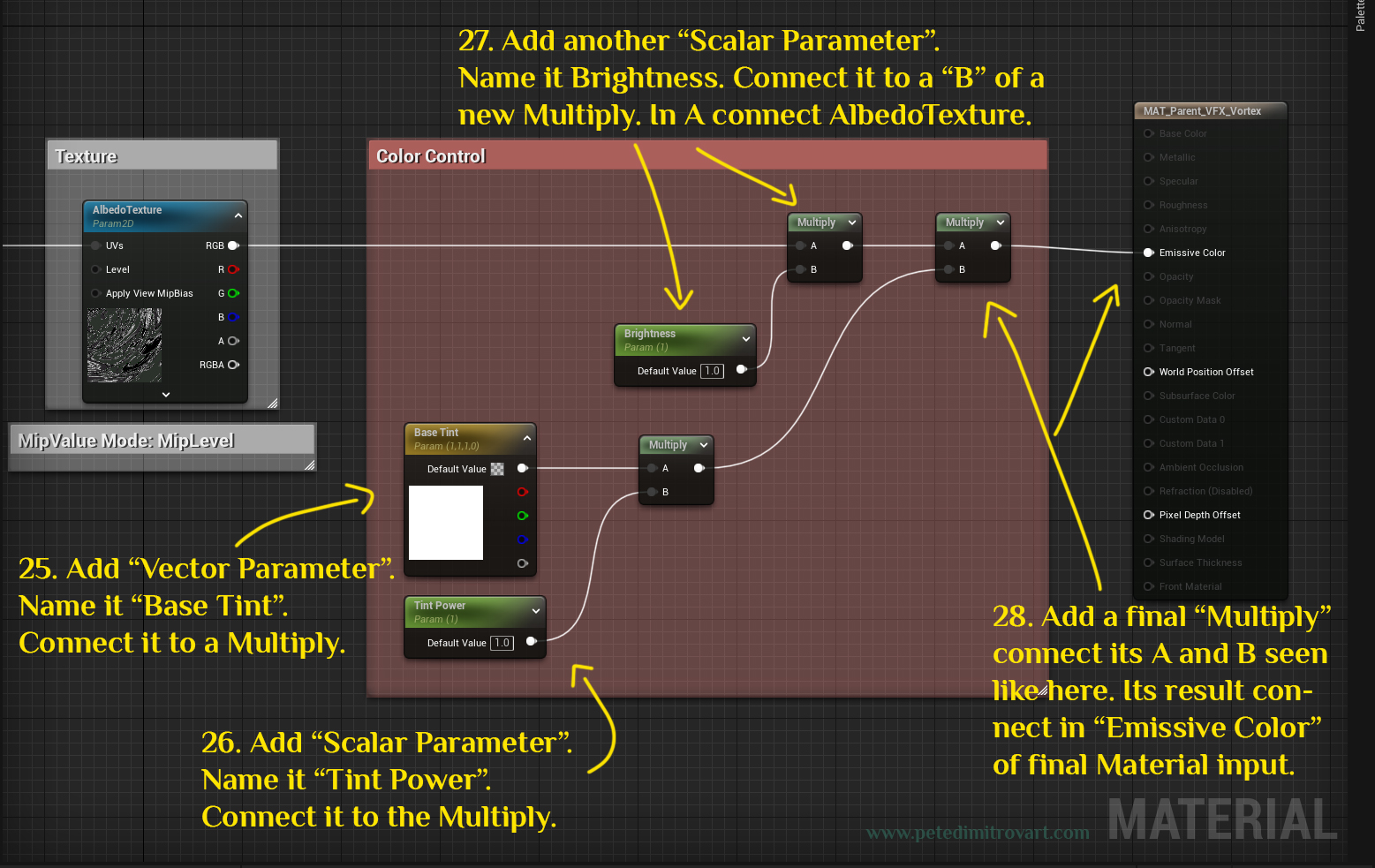
Start by adding a “Vector Parameter”. Name it “Base Tint”. Connect it to a new Multiply. Then add a new “Scalar Parameter”. Name it “Tint Power”. Connect it to the Multiply as well.

Add another “Scalar Parameter”. Name it “Brightness”. Connect it to the “B” of a new Multiply node. In the A connect the AlbedoTexture node from the previous steps.

Add a final “Multiply”. In the A input of it, add the previous “Multiply”. In the B, add the “Multiply” that comes right after the “Base Tint” color node (vector parameter). The result of this final “Multiply”, connect into the “Emissive Color” of the final Material Input.

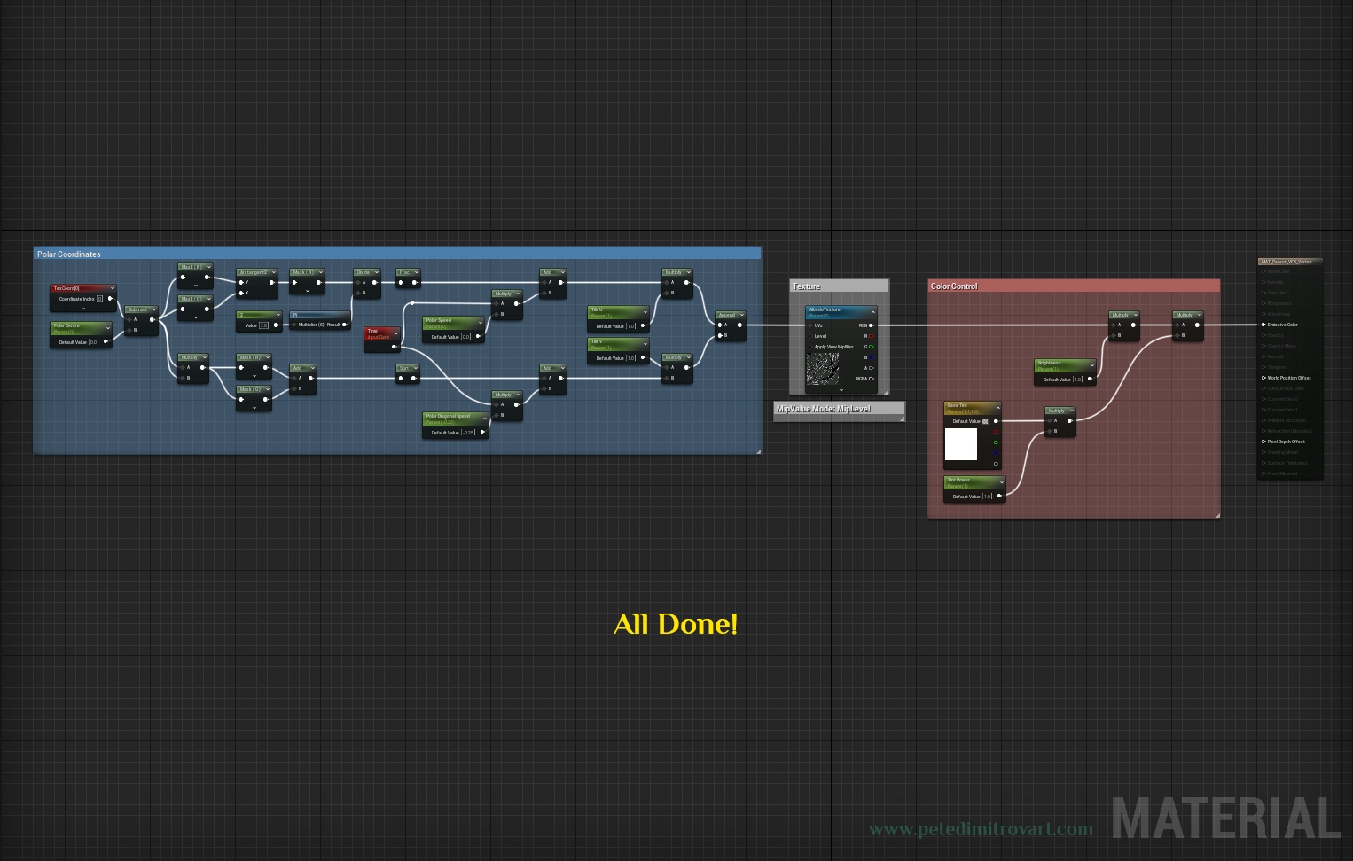
(When you are done with all of the above you can select it all and add yourself a red comment frame, like seen below. Name it “Color Control”.)

Screenshot that shows the nodes that come right after the “Texture” group shown in gray in the previous image. The arrows point to new Vector Parameter called “Base Tint” as well as few new scalar parameters called “Tint Power” and “Brightness” they are all connected through few multiplies. Text explaining is transcribed in paragraph above.

We are all done! Zoom out and take a look at all of it.

The entire material graph board, zoomed out, seeing it all. Yellow text underneath reads “All Done!”.

Material Instance

Go back to your Project Directory. Find where this material parent that we just made is. Right click on it and select “Create Material Instance”. Call it “MAT_VFX_Vortex_A”. Open it. All of the Scalar Parameters and Vector Parameters (color) have default values but we now want to connect our texture in there and also change the values so we get the visual we want.

Parameters

After opening the newly created material instance, use the parameter values as seen here:

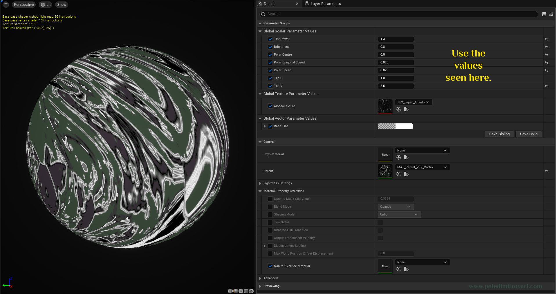
Screenshot of an open Material Instance window in Unreal 5. To the left is a preview of the texture, displayed on a ball. Looks like white, gray liquid spill. On the right are the Parameter Groups and all of the scalars, vectors and texture settings. Those are transcribed below.

Tint Power: 1.3

Brightness: 0.8

Polar Centre: 0.5

Polar Diagonal Speed: 0.025

Polar Speed: 0.02

Tile U: 1.0

Tile V: 3.5

Albedo Texture: TEX_Liquid_Albedo (this is the black and white texture we made in the previous tutorial)

Base Tint: FFFFFF00 (white color)

Preview in Action

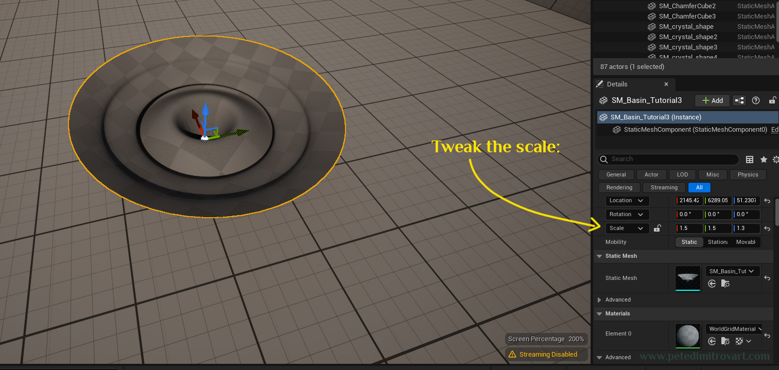
Drag into a scene the imported vortex geometry you created in part one of the tutorial. Then change its scale to 1.5 1.5 1.3 (this is optional, I just scaled mine a bit so its not too small when compared to a 2m tall human mannequin).

Opened Unreal 5 blank scene screenshot. The floor is seen in a checkerboard material. Above is placed a vortex VFX static mesh. Arrow points to its scale settings that are changed to X 1.5 Y 1.5 and Z 1.3.

Then change the material settings. Select the Material Instance we created - “MAT_VFX_Vortex_A”.

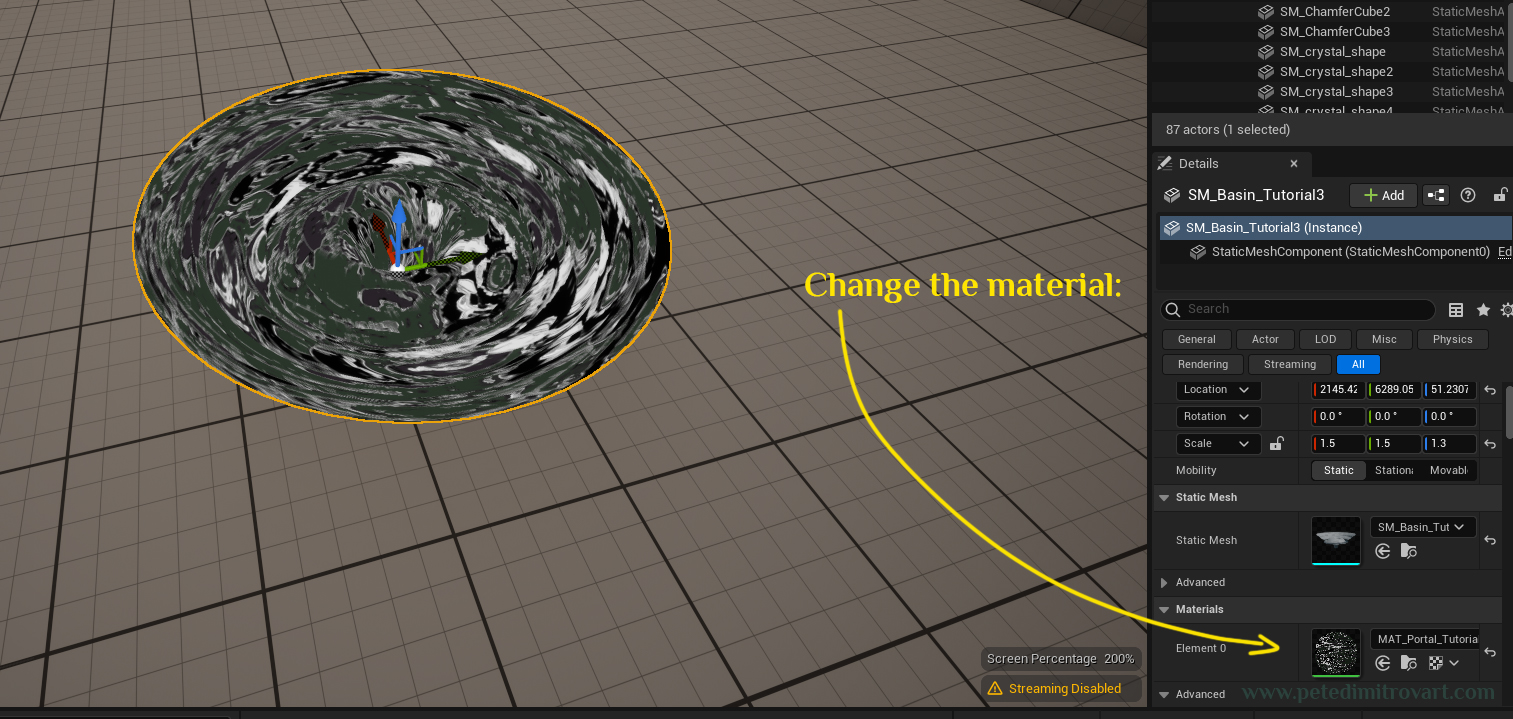
Same angle and subject as before, but this time around the vortex static geometry has its material changed. As such the shading on it is now as a liquid, gray VFX.

Congrats! This is it. You should be able to see the movement and animation in the VFX.

Troubleshooting

If you dragged your material shader onto the geometry and your object suddenly turned pitch black, then lets fix that.

This most commonly happens on older versions of UE.5. Its due to the material graph parent shader not being suitable for “Nanite Geometry”.

Remove the imported static geometry vortex basin from the project directory (content browser). Now re-import it but this time around from the Import settings tick “Nanite” off. Now retry dragging it into the scene and applying the material and it should work.

Important:

If you look at the VFX result from a camera angle from above, you will see UV distortion imperfection. We resolve that in the next part of the tutorial. Even if you don't want to create a refraction shader, and would like to skip that, make sure to still visit the next tutorial and find the solution to this UV distortion issue.

Next part in the tutorial where we can see the solution to fixing the UV distortion in the middle. Scroll down to the “Troubleshooting” chapter in there to see it.

Color

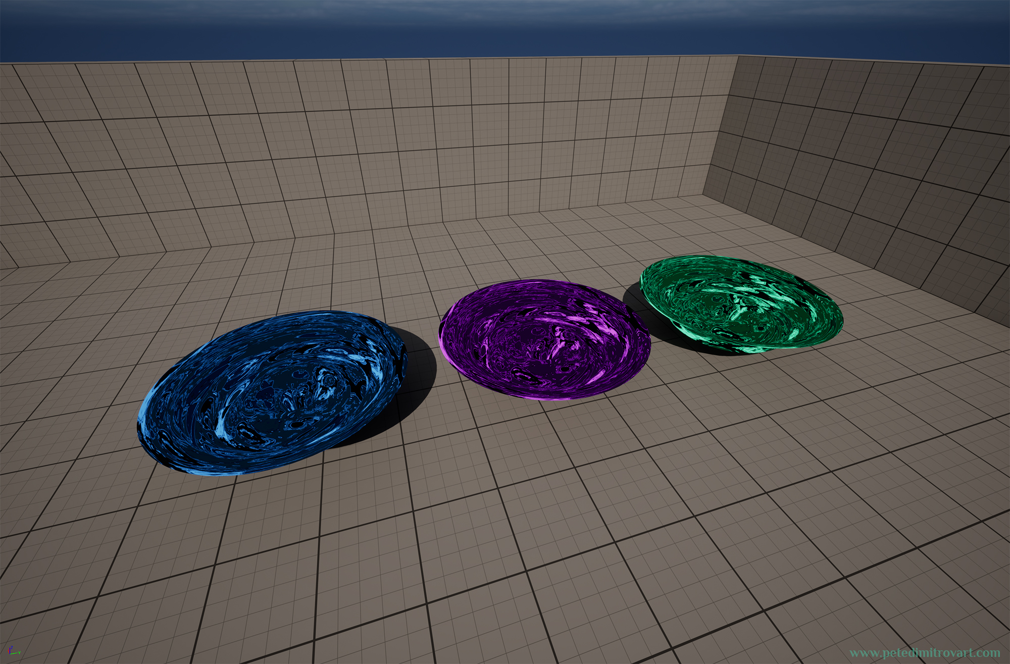
We keep it to white here because in the final part of the tutorial series, we will create a Blueprint in which we control the color tint. That part is optional. As such if you prefer to skip it, and instead want the colors right away, as seen in the tutorial previews (blue, purple, green), then do the following.

Create 3 copies of the above material instance. That is the one we just made and called “MAT_VFX_Vortex_A”. Those copies rename “MAT_VFX_Vortex_Blue”, “MAT_VFX_Vortex_Purple” and “MAT_VFX_Vortex_Green”. Go in each and change the “Base Tint” HEX linear value.

Blue: 1A5CF700

Purple: 941AF700

Green: 1AF78100

UE5 scene screenshot. Displays the end result of the color settings above. Three vortex basins sit onto a gray placeholder floor. They are blue, purple and green in color tint and have the liquid-metal patterns and distortion we are after.

Conclusion

In this tutorial we created the main driving force of the VFX: the polar coordinates shader. We then created material instances of it and went over what settings to use in order to get the visual we want.

In the next part of the series, we will quickly create a “Refraction” material shader. We will use that as a floating layer of detail, above the vortex we have now. This step will be incredibly short and easy to make in comparison to the length and difficulty of the previous 3 parts of this tutorial.

Next part in the tutorial - Creating Refraction Material Graph. Adding it as a layer of detail on the vortex.

Bibliography

Arctan - Math Open Reference

Animating UV Coordinates - Unreal Engine Documentation

Math Material Expressions - Unreal Engine Documentation

Polar and Cartesian Coordinates… and how to convert between them.

Polar Coordinates Node Description - Unity Documentation

Cheers,

Pete.

If you enjoyed this blog post, consider subscribing in the form below. That way you will get a notification the next time I publish a new blog.